Convert a hotspot grid to isobands

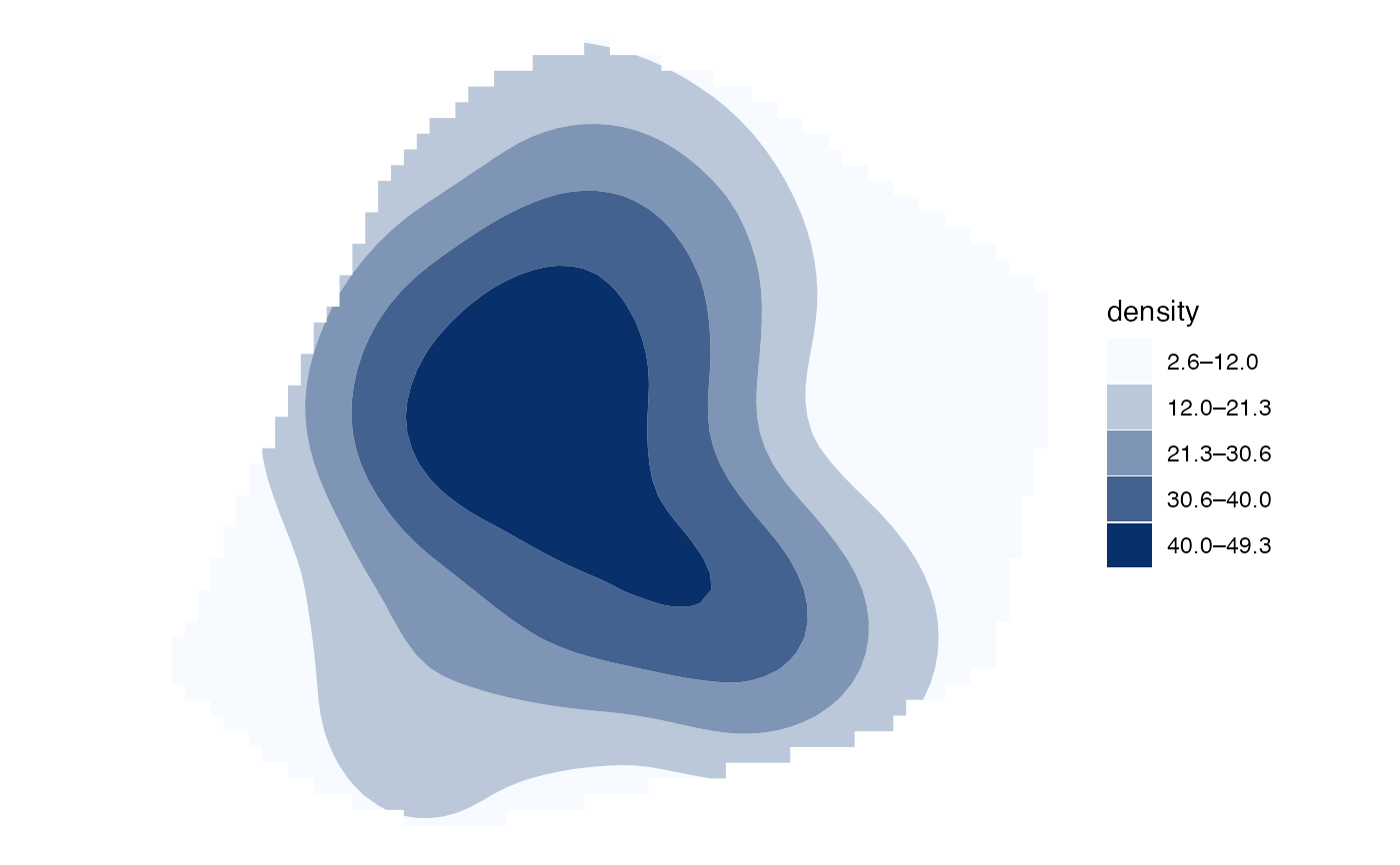
Generalise values in a regular square grid into polygon bands. The result is an sf::sf object with one row for each non-empty band and can be plotted with autoplot() or hotspot_layer().

Usage

hotspot_isoband(
  data,
  value = NULL,
  breaks = 5,
  style = "equal",
  critical_p = 0.05,
  quiet = FALSE
)

Arguments

data

An sf::sf object containing a regular square grid and at least one numeric column, typically produced by a hotspot_*() function.

value

The unquoted name of the numeric column to convert. If NULL, a suitable column is inferred from the sfhotspot class of data, or from the sole numeric column in an otherwise unrecognised SF object.

breaks

Either a single positive integer giving the requested number of bands (five by default), or a strictly increasing numeric vector giving the band boundaries. If multiple boundaries are supplied, style is silently ignored.

style

Method used to calculate breaks when breaks has length one. Values other than "pconventions" are passed to the style argument of classInt::classIntervals(). "pconventions" uses two-sided normal-theory thresholds corresponding to p-values of 0.1, 0.05, 0.01 and 0.001 and ignores breaks.

critical_p

For output from hotspot_gistar() containing a kde column, the largest p-value for a cell to be included. The default is 0.05. This argument is ignored for other inputs.

quiet

If TRUE, suppress informative messages about automatically selected values and potentially unhelpful intervals.

Value

An sf tibble with class hspt_ib. It has one row per non-empty band and columns lower, upper, band, label, and geometry. The band and label columns are ordered factors; band contains technical interval notation and label contains ranges formatted for display.

Details

The default style = "equal" divides the observed range into equal-width intervals, providing a discrete analogue of a linear continuous colour scale. Extreme values can make equal-width bands uninformative; a message is produced when at least 90% of finite values fall in one calculated band.

For change values, Gi*/Gi statistics, and dual-KDE differences or logged ratios, automatically calculated breaks place zero at a boundary or at the centre of a band. Explicit break vectors are never altered.

When data is output from hotspot_gistar() and contains KDE values, KDE is converted and cells with pvalue >= critical_p are excluded before the bands are calculated. Without KDE values, the Gi*/Gi statistic is converted.

Values are interpolated between grid-cell centres. Lattice positions absent from a grid clipped to its original analysis area are treated as missing. Consequently, the isobands need not cover the complete area of every outer grid cell.

Examples

# \donttest{
memphis_robberies_jan |>
  hotspot_kde() |>
  hotspot_isoband() |>
  autoplot()
#> Cell size set to 0.00512 degrees automatically
#> Data transformed to "WGS 84 / UTM zone 16N" co-ordinate system.
#> ℹ CRS code: "EPSG:32616".
#> ℹ Unit of measurement: metre.
#> Bandwidth set automatically based on rule of thumb.
#> ℹ Bandwidth = 8,867 metres.

# }